Chapter 3 Methods

3.1 Geolocation

Light-level geolocators were deployed on adult male Rosefinches in Finland, Sweden, Germany, Czechia and Bulgaria (Table 1). In Finland, geolocators were deployed at different filed sites during 2015 (SOI GDL2 n = x) and 2016 (SOI GDL2 n = x and Migrate Technology Intigeo XX n = x). In Sweden, birds were captured and equipped with geolocators in 2011 (Halland, BAS BAS Mk12S n = 10), 2012 (Gotland, MT Intigeo-P65 n = 4; Halland, MT Intigeo n = 2) and 2013 (Gotland, MT Intigeo-P65 n = 21). In Germany, initial fieldwork took place at one site during 2013 (Margrafenheide, SOI GDL2 n =20). At two sites in Czechia, geolocators were put on Rosefinches in 2012 (Želnava, MT Intigeo P55, n = 10; České Milovy, MT Intigeo P55, n = 4) and 2013 (České Milovy, SOI GLD2 n = 20). In Bulgaria, geolocators were deployed in 2012 (MT Intigeo P55, n = 8) and 2013 (MT Intigeo P55, n = 6) at Razlog-Bansko. At all sites, birds were caught at their breeding locations using mist nets. All individuals were individually marked (metal ring and color bands), measured and equipped with a geolocator mounted on a leg-loop harness. Geolocators with the harness weighted between 0.6 and 0.8 g, which represents 4.1 to 2.6 % of the body mass. Thus, we expect no or very minor effects on the individuals behavior and fitness due to the extra weight of the device Brlik et al. 2019.

We used a threshold approach Lisovski et al. 2019 to estimate locations from the light-level data using the R packages TwGeos Lisovski et al. 201, GeoLight v2.01 Lisovski and Hahn 2012 and SGAT Wotherspoon et al. 2013. In short, sunrise and sunset events were identified using a light intensity threshold of 0.8 arbitrary values for the SOI GDL2 and 0.5 lux for MT Intigeo as well as for BAS Mk models. Calibration was conducted for all tags separately using the maximum number of days recorded at the breeding sites after logger deployments. Next, we applied the invChanges function from GeoLight to identify changes in sunrise and sunset times and distinguish between movement and stationary periods. Based on this analysis, we assigned twilight events to either a stationary period (only for periods that were found to include at least three days) or to movement. We used the group method in SGAT to estimate location. SGAT uses a Bayesian framework to incorporate prior information including the assigned stopover periods, twilight error distribution (parameters from the calibration), speed distribution (gamma distribution with shape = 2.2 and scale = 0.08) and a land mask (so that when the bird stops over, it is less likely to do so in the sea). During a Markov Chain Monte Carlo simulation, the geographical probability distribution was calculated for each twilight times during movement and for each stationary period. Providing stationary periods and thereby grouping twilight times and estimate a single location from all sunrise and sunset events that belong to the same stationary period helps finding the best possible fit to the data during this period, and importantly, increasing the precision of the estimated location. We fixed the first and, if the bird was still recording in spring, last location to the known capture and recapture locations where appropriate. We first ran a modifiedGamma model (relaxed assumptions) for 1000 iterations to initiate the model, before tuning the model with final assumptions/priors (three runs with 300 iterations). Finally, the model was run for 2000 iterations to ensure convergence. From the resulting 2000 chains, we extracted median location estimates for each twilight during movement and for each stationary period including the 95% credibility interval.

3.2 Simulations

3.2.1 Spatial Grid

For the simluations on optimal wind selection and optimal resource tracking by migrating songbirds along the Flyway, we used a hexagonal grid, allowing to distribute the nodes roughly equally across the investigated area (0.0° - 89.0° W, 5.0° - 72.0° N).

Figure 3.1: Spatial Grid with hexagonal grid-cells sourrounding the same area (e.g. equal distance between mid-points).

We chose five breeding locations representing locations from the five Common Rosefinch populations we tracked to their wintering sites. To keep the simulations simple we choose five locations that roughly represent the spread of the wintering sites of the tracked Rosefinches.

Figure 3.2: Breeding (cicles) and wintering sites (diamonds) used in the simulations.

3.2.2 Wind

To investigate optimal routes in terms of wind efficiency across all five Rosefinch populations, we followed the general approach established by Kranstauber et al. (2015). In short, our model calculates the fastest route between the breeding locations (five major locations) and four locations across the wintering range, traveling over a grid consisting of 229 cells or nodes (see section Spatial Grid). Travel is allowed along straight connections to the six surrounding cells and the second-order neighbours creating 12 travel connections about 30° apart. The distance to the direct neighbour was on average 150 km, and 300 km respectively. Wind data was provided by the European Centre for Midrange Weather Forecast (ECMWF; https://www.ecmwf.int/). For the interpolation of wind, we used three layers of the atmospheric model, 925, 850 and 700 millibar, which correspond to the median altitude of 779, 1502 and 3130 meters above sea level. These altitudes cover the range where most migration is observed in radar and recent geolocator studies (Kemp et al. 2013, Liechti et al. 2018, Dhanjal-Adams et al. 2018). The model begins from a starting location and initiates travel to all surrounding nodes. Travel time to the nodes depends on the ground speed (vg) that was calculated as a function of cross wind (wc) wind support (ws) and air speed (10 ms-1). For each time step of 3 hours, the wind conditions from the altitude with the best supporting winds (or least crosswind) was chosen, assuming that birds regularly change altitude during flight (Liechti et al. 2018). This process continues and reiterates until the destination is reached.

Figure 3.3: A visualisation of the algorithm that finds the optimal route. Travel starts at the grey node in all directions without intended destination. Wind is indicated by the arrow at the blue points. The air speed of the bird in each direction is kept constant at 10 m s?1. The realised ground speed indicated by the black circle, however, is influenced by wind speed and direction which are interpolated bi-linearly to all nodes. When a node has been reached (solid circles), the travel continues from there iterating the calculations by travelling to all surrounding nodes that have not yet been reached. Inclusion of the influence of wind on the ground speed results in the optimal routes (thick lines) to many nodes actually not being the direct connection. This algorithm is repeated until all locations are reached thus providing the quickest route to all location on the grid. Figure adopted from Kranstauber et al. (2015).

This algorithm finds the shortest route in our hexagonal grid from the starting point to all locations on the grid. The distances in the grid are determined by travel time calculated using the speed function described in Kranstauber et al. (2015). We calculated the optimal route from all five wintering locations to all five breeding locations, and vice-versa, starting every 5th day between 1 April and 31 May in spring and 1 August and 31 September in autumn across 2012 to 2017. This resulted in 60 routes per population and year. To weight routes, we used the same approach described by Kranstauber et al. (2015), namely, to calculate travel time throughout the study period at the same starting date over the optimal routes. We than assume that travel time (t) has a sigmoidal relation with mortality and calculated an average survival per year for each route using the travel time across all years:

\[\phi_{Wind} = 1 - \frac{t^2}{\lambda - t^2}\]

Where \(\lambda\), the migration mortality is set to the mean travel time across all years squared for every location pair (combination) and starting date separately. This means, on an average migration between two locations half of the individuals would die. The geometric mean of \(\phi\) represents this the average survival of a route over the study period as the nth root of the product of all survival probabilities (where n is the number of years survival has been measured).

3.2.3 Resources

To investigate routes that provide some level of resources along the way and optimise prospective survival, we used a similar procedure as described for the wind simulation with normalized differenced vegetation indices (NDVI) as the underlying environmental variable. Weekly NDVI layers with a 4 km resolution were downloaded from NOAA (https://www.star.nesdis.noaa.gov/smcd/emb/vci/VH/vh_ftp.php). NDVI values differ between 0 and 1 and indicate levels of photosynthetic activity. It has been shown that this correlates well with primary productivity and to some extent higher trophic level productivity Pettorelli et al. 2005. Many terrestrial migratory birds including Common Rosefinches, mainly fly during the night and rest during the day (). Furthermore, they cannot cover the entire distance without extended (>1 day) stopping periods during which they replenish their fuel loads. For this, they need to stop at suitable locations. We here assume, that individual birds can fly approximately 10 hours per day with have an average ground speed of 15 meters per second (). Thus, they can travel up to 540 km per day. During the migration periods simulation started on the same days as described in the wind simulation. For each wintering site in spring, breeding site in autumn and for all dates, an individual Rosefinch starts (t=0) by calculating the prospective survival for all sites that are in reach during the next nights flight period (sites <= 550 km away). The prospective survival was based in the NDVI value for the grid cell following a sigmoidal relation:

\[\phi_{NDVI} = \frac{1}{1 - e^{a-(x-b)}}\]

with parameters a = 20 and b = 0.3 resulting in zero survival for NDVI = 0 and a survival of 0.5 for NDVI = 0.3.

Figure 3.4: Relationship between prospective survival and NDVI values used in the simulations.

In the next time step (t=1), the individual starts from the grid that provided the highest prosp. survival. Unlike in the previous step, only cells that are in reach and are not yet evaluation during the previous round are considered as potential destinations. The prospective survival for these cells is again based on the NDVI for this timestep, however, multiplied by the prosp. survival of the origin (e.g. the highest prosp. survival of t=0). This process is repeated until all cells have been reached, allowing a path construction from all breeding sites (or vice versa in autumn) to the starting point that indicates the paths with the highest possible prosp. survival for this date.

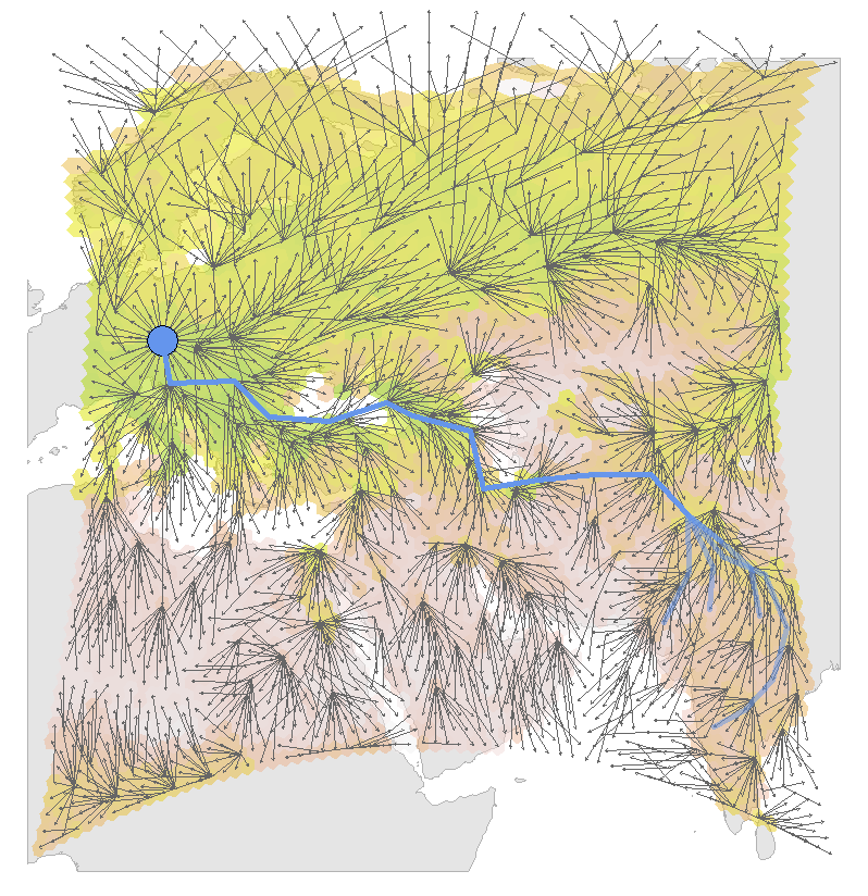
Figure 3.5: Example of the simulation results for one date and one breeding population (CZE). The bakcground colors indicate the maximum NDVI values for each grid cell at this date (2012-09-01). The arrows indicate possible flight bouts. The blue lines are the resulting tracks, based on the possible flight bouts and the maximized prospective survival for each wintering site.

Both models were implemented in R (Version 3.5.0).